Classifying Astronomical Data Using Tree Based Methods
The following is a guide to using tree based methods in R, based on the corresponding chapter in ‘An Introduction to Statistical Learning’ but using data from the Sloan Digital Sky Survey (SDSS). The aim is to use the five colour bands provided by the SDSS extract, u (ultraviolet), g (green), r (red), i & z (very-near-infrared), to predict whether the sources in the survey are Quasars, Stars or White Dwarfs. I use a variety of techniques, from simple decision trees to ensemble methods such as random forests.
Data
Rather than getting the data directly from SDSS and doing the cleaning myself, I’m going to cheat and use a pre-filtered data set used in the book ‘Modern Statistical Methods for Astronomy’, available here. As part of their extract they perform a few cleaning operations, such as ignoring spatially resolved galaxies, those with large measurement errors, and those that are very bright (and could cause saturation) or very faint (with uncertain measurements). They also provide 3 labelled data sets for training, one each for Quasars, Stars & White Dwarfs.
The colour bands as they stand aren’t particularly useful, since objects of the same class can be at different distances, and therefore have relatively lower flux across all bands. This can be avoided by looking at the ratios of brightness across bands, and since magnitudes are logarithmic units of brightness we simply find the difference between the provided values to get four colour indices, (u-g), (g-r), (r-i) & (i-z).
The following three code chunks extract and clean the training data for all three sources and combine them in to a single data frame. Quasras, stars and white dwarfs are given the labels 1,2 and 3 respectively. There are 5000 stellar objects available for training, but for quasars there are over 7.7429 × 10⁴ and for white dwarfs over 1.009 × 10⁴, so I’ve filtered each of the latter two down to only 5000 so that there are equal numbers of each class.
Quasar training set (Class 1):
dat1 <- read.table('http://astrostatistics.psu.edu/MSMA/datasets/SDSS_QSO.dat', h=T)
bad_phot_qso <- which(dat1[,c(3,5,7,9,11)] > 21.0 | dat1[,3]==0)
dat1 <- dat1[1:5000,-bad_phot_qso,]
dat1 <- cbind((dat1[,3]-dat1[,5]), (dat1[,5]-dat1[,7]), (dat1[,7]-dat1[,9]), (dat1[,9]-dat1[,11]))
qso_train <- data.frame(cbind(dat1, rep(1, length(dat1[,1]))))
names(qso_train) <- c('u_g', 'g_r', 'r_i', 'i_z', 'Class')
Star training set (Class 2):
dat2 <- read.csv('http://astrostatistics.psu.edu/MSMA/datasets/SDSS_stars.csv', h=T)
dat2 <- cbind((dat2[,1]-dat2[,2]), (dat2[,2]-dat2[,3]), (dat2[,3]-dat2[,4]),
	(dat2[,4]-dat2[,5]))
star_train <- data.frame(cbind(dat2, rep(2, length(dat2[,1]))))
names(star_train) <- c('u_g','g_r','r_i','i_z','Class')
White dwarf training set (Class 3):
dat3 <- read.csv('http://astrostatistics.psu.edu/MSMA/datasets/SDSS_wd.csv', h=T)
dat3 <- na.omit(dat3)
dat3 <- cbind((dat3[1:5000,2]-dat3[1:5000,3]), (dat3[1:5000,3]-dat3[1:5000,4]),(dat3[1:5000,4]-dat3[1:5000,5]), (dat3[1:5000,5]-dat3[1:5000,6]))

wd_train <- data.frame(cbind(dat3, rep(3, length(dat3[,1]))))
names(wd_train) <- c('u_g', 'g_r', 'r_i', 'i_z', 'Class')
Combine the training sets
SDSS_train <- data.frame(rbind(qso_train, star_train, wd_train))
names(SDSS_train) <- c('u_g', 'g_r', 'r_i', 'i_z', 'Class')
str(SDSS_train)
## 'data.frame': 15000 obs. of 5 variables:
## $ u_g : num -0.079 0.033 0.11 0.325 0.22 ...
## $ g_r : num 0.136 0.255 0.425 0.448 0.049 ...
## $ r_i : num 0.233 0.454 0.221 0.114 0.189 ...
## $ i_z : num 0.046 0.3 -0.158 0.221 0.04 ...
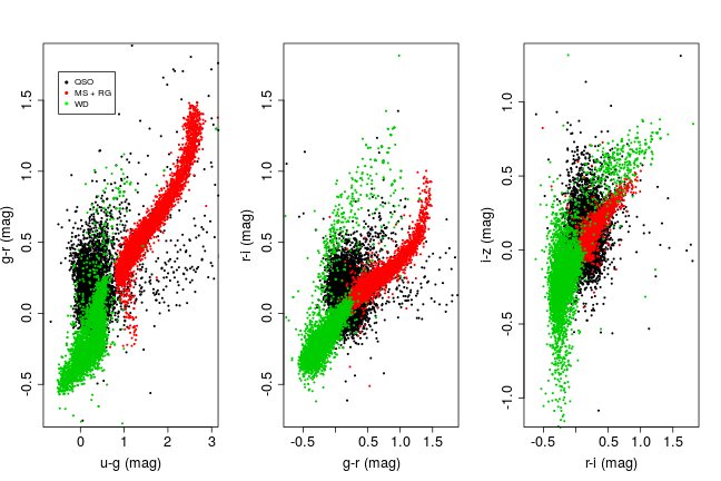
## $ Class: num 1 1 1 1 1 1 1 1 1 1 ...The plot below shows each training class on a bivariate colour-colour scatter plot.There’s plenty of structure to each class, something that tree based methods should be more than capable of picking up on.
Decision Trees
Decision trees are the most basic tree based method, and one on which the majority of other methods are built on They work by splitting the predictor space in to regions; each split can be thought of as a branch, and each of the remaining regions are leaves.
The default tree library has a simple binary recursive partitioning method for growing regression or classification trees.
library(tree)Below we split the data in to a training and test set, and train the classifier on the training test.
SDSS_train$Class <- as.factor(SDSS_train$Class)

set.seed(1)
train <- sample(nrow(SDSS_train), 4*nrow(SDSS_train)/5)

tree.sdss <- tree(Class~., data = SDSS_train, subset = train)
tree.sdss is our trained classifier. We can plot it to see the major branches and leaves of the tree. The default is pretty cluttered, so I’ve coloured and rotated the text to make it easier to read… not sure if that really helps. The rpart package for building trees has some nicer plotting capabilities but, in the spirit of every undergraduate lab report, ‘that is beyond the purposes of this investigation’.
plot(tree.sdss)
text(tree.sdss,col=rainbow(10)[1:25],srt=35,cex=0.8)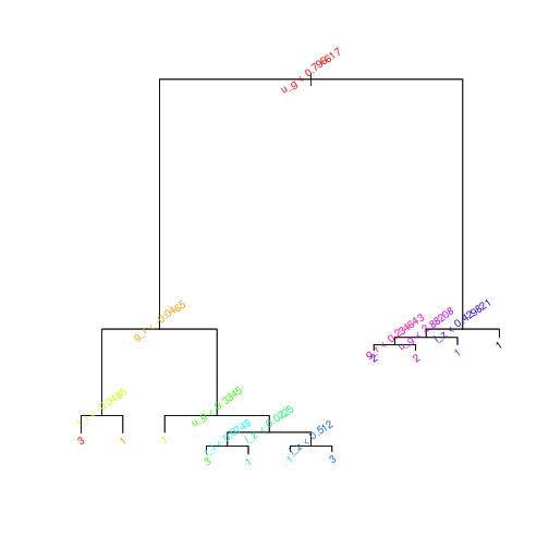
To evaluate our tree, we use it to predict the class of our test data.
tree.pred <- predict(tree.sdss, SDSS_train[-train,], type="class")Below is a confusion matrix of the predicted classes against the actual.
##
## tree.pred   1   2   3
##         1 921   8 131
##         2  65 985   1
##         3  14   0 875
The overall test error rate is 7.3%.
Often the algorithm that builds the tree can create more branches than necessary, and end up reducing the predictive accuracy of our classifier. To test this I perform cross validation on the built tree. Specifying FUN = prune.misclass tells cv.tree that we want the cross validation to be guided by the classification error rate, rather than the default which is the deviance.
cv.sdss <- cv.tree(tree.sdss, FUN = prune.misclass)
cv.sdss
## $size
## [1] 11 10 9 7 6 5 3 2 1
##
## $dev
## [1] 868 868 922 971 1039 1194 1592 4050 8177
##
## $k
## [1] -Inf 0.0 38.0 44.5 72.0 111.0 217.0 2482.0 3943.0
##
## $method
## [1] "misclass"
##
## attr(,"class")
## [1] "prune" "tree.sequence"The left hand plot shows the error rate against tree size, the right against the cost complexity parameter k.
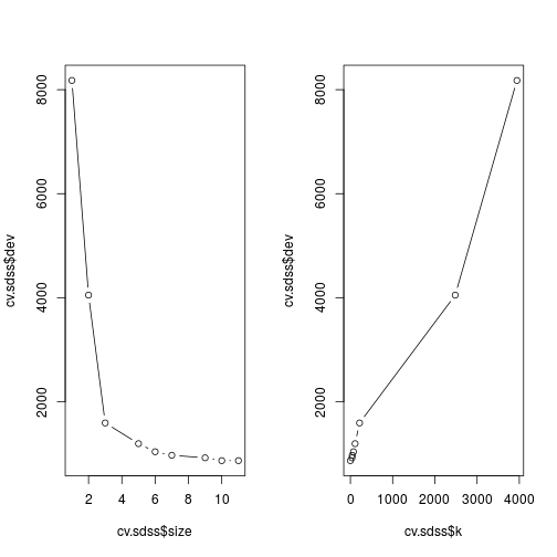
The 10 branch tree has the same error rate as the 11, so pruning to this size will not reduce the predictive power of the model, but will reduce the complexity.
min_size = cv.sdss$size[max(which(cv.sdss$dev == min(cv.sdss$dev)))]  # find minimum size that fits best

prune.sdss <- prune.misclass(tree.sdss, best = min_size)
par(mfrow=c(1,1))
plot(prune.sdss)
text(tree.sdss,col=rainbow(10)[1:25],srt=35,cex=0.8)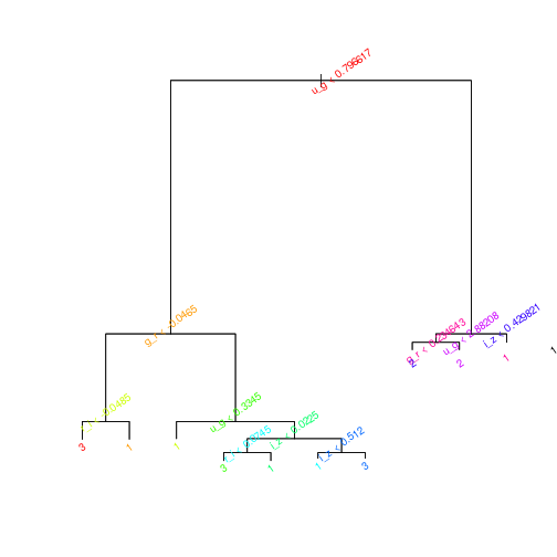
tree.pred <- predict(prune.sdss, SDSS_train[-train,], type="class")

test.results <- table(tree.pred,SDSS_train[-train,"Class"])
test.results
##
## tree.pred 1 2 3
## 1 921 8 131
## 2 65 985 1
## 3 14 0 875The error rate, 7.3%, is the same, as expected, but the tree is easier to interpret.
Bagging and Random Forests
Bagging and random forests are both examples of ensemble methods, where many decison trees are combined together to improve the prediction accuracy. Both can be implemented using the randomForest package.
Bagging (derived from the full name Bootstrap Aggregation) takes multiple bootstrapped samples from the same training set and builds an ensemble of trees that are then averaged. Bagging uses all predictors; mtry states that all 4 predictors should be considered for each split of the tree.
library(randomForest)bag.sdss <- randomForest(Class~., data = SDSS_train, subset = train, mtry = 4, importance = T)
bag.sdss##
## Call:
## randomForest(formula = Class ~ ., data = SDSS_train, mtry = 4, importance = T, subset = train)
## Type of random forest: classification
## Number of trees: 500
## No. of variables tried at each split: 4
##
## OOB estimate of error rate: 2.38%
## Confusion matrix:
## 1 2 3 class.error
## 1 3853 55 92 0.036750000
## 2 25 3981 1 0.006488645
## 3 111 1 3881 0.028049086yhat.bag <- predict(bag.sdss, newdata = SDSS_train[-train,])##
## yhat.bag 1 2 3
## 1 966 5 36
## 2 12 988 0
## 3 22 0 971The test error rate associated with the bagged tree is 2.5%, a significant improvement over the single decision tree.
Random forests are similar to bagged trees, but with a small tweak to the algorithm; at each step, when a split is considered only a random subset of the predictors is made available. This prevents strong features from dominating the root branches of the trees, otherwise this can lead to correlations between the predictions of the trees, as they all look relatively similar. The trees in a random forest ensemble can be thought of as decorrelated.
Growing a random forest proceeds in the same way as Bagging, but with a smaller value for mtry. By default, for classification problems randomForst uses $\sqrt{p}$ predictors, so 2 in our case.
rf.sdss <- randomForest(Class~., data = SDSS_train, subset = train, importance = T)
rf.sdss
##
## Call:
## randomForest(formula = Class ~ ., data = SDSS_train, importance = T, subset = train)
## Type of random forest: classification
## Number of trees: 500
## No. of variables tried at each split: 2
##
## OOB estimate of error rate: 2.17%
## Confusion matrix:
## 1 2 3 class.error
## 1 3869 50 81 0.032750000
## 2 23 3983 1 0.005989518
## 3 104 2 3887 0.026546456yhat.rf <- predict(rf.sdss, newdata = SDSS_train[-train,])
test.results <- table(yhat.rf, SDSS_train[-train,"Class"])The test error rate associated with the random forest is 2.37%, a further improvement over the bagged tree.
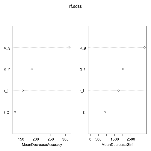
We can use the importance function to view the importance of each of the variables used as our features. The first, %IncMSE, measures the mean decrease in accuracy of the predictions on out of bag samples when that feature is excluded from the model. The second, IncNodePurity, measures the decrease in node impurity due to splits over that variable, over all trees; node impurity measured by training RSS in the case of regression trees, and deviance for classification trees. varImpPlot plots these importance functions.
Boosting
Boosting algortihms for regression and classification problems are different, and I will not provide a full description here (for details, see here). In basic terms, boosting algorithms apply many weak learners sequentially to the residuals (i.e. the remaining unexplained data) of previous trees. The algorithm learns slowly and incrementally, which can lead to a better resulting model, at the cost of extra computation compared to more direct learners.
The gbm function, from the identically named package, is used here to perform Boosting.
boost.sdss <- gbm(Class~., data = SDSS_train[train,], distribution = "multinomial", n.trees = 5000, interaction.depth = 4)summary(boost.sdss)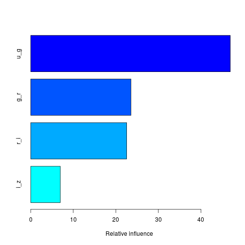
##     var   rel.inf
## u_g u_g 46.908265
## g_r g_r 23.571429
## r_i r_i 22.557859
## i_z i_z  6.962446
The plot above shows the relative importance of each feature in the training data. The interaction.depth argument, in the cal to gbm, limits the depth of each tree. Here we use a multinomial distribution as this is a multinomial classification problem; if it was binary, use a bernoulli distribution, or if performing a regression, use a gaussian distribution.
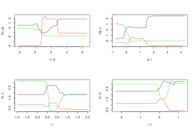
Below are some partial dependence plots, which integrate out other variables to show the marginal effect of selected variables. The black line shows class 1, the red line class 2, and green class 3 (Quasars, Stars & White Dwarfs respectively). The peaks of each line show where for this line ratio that particular class can be identified most clearly.
yhat.boost <- predict(boost.sdss, newdata = SDSS_train[-train,], n.trees = 5000, type='response')
yhat.boost <- apply(yhat.boost, 1, which.max) # find max predictor
##
## yhat.boost 1 2 3
## 1 953 3 47
## 2 28 990 0
## 3 19 0 960Test error rate associated with Boosting is 3.23%. This is actually worse than the bagging and random forest approaches above, for this particular data set, and the performance is $~\mathcal{O}(10)$ worse.
Extremely randomized trees
Extremely Randomised Trees (ERTs) are a relatively modern incarnation of random forests. The difference is that, after choosing a random subset of features, the threshold for the split on each feature is also chosen randomly, and the best split is then chosen. Then ensemble of trees is again combined to provide the best estimate. This randomness increases the variance at the cost of a little bias.
The extraTrees package in R can execute ERTs. Somme of the documentation looks a little rough around the edges, so I’d certainly take a closer look at the source code if you’re doing anything important with it. For our purposes though it will suffice.
library(extraTrees)et <- extraTrees(SDSS_train[train,-5], SDSS_train[train,"Class"])
yhat.et <- predict(et, SDSS_train[-train,-5])##
## yhat.et 1 2 3
## 1 972 3 35
## 2 12 990 0
## 3 16 0 972Test error rate associated with ERTs is 2.2%, the best of all the approaches demonstrated here.
SDSS ‘test’ data
The source of the data used in this post, the textbook ‘Modern Statistical Methods for Astronomy’, made another set of SDSS data available named ‘test data’ that consist of 17000 sources. Unfortunately it doesn’t have any associated source classes, making it a pretty useless test set! However, it is useful to apply our models to and analyse from inspection. Here I use the random forest model, since it has one of the best error rate to complexity ratios. Below is a colour-colour plot similar to that made at the start of the workbook for the training data (repeated below for easier comparison).
SDSS point sources test dataset, N=17,000 (mag<21, point sources, hi-qual)
SDSS <- read.csv('http://astrostatistics.psu.edu/MSMA/datasets/SDSS_test.csv', h=T)
SDSS_test <- data.frame(cbind((SDSS[,1]-SDSS[,2]), (SDSS[,2]-SDSS[,3]),
	(SDSS[,3]-SDSS[,4]), (SDSS[,4]-SDSS[,5])))
names(SDSS_test) <- c('u_g', 'g_r', 'r_i', 'i_z')SDSS_test$Class.Predict <- predict(rf.sdss, SDSS_test)
#yhat.boost <- predict(boost.sdss, SDSS_test, n.trees = 5000, type='response')
#SDSS_test$Class.Predict <- apply(yhat.boost, 1, which.max) # find max predictor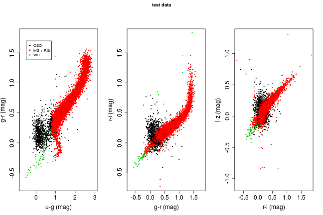
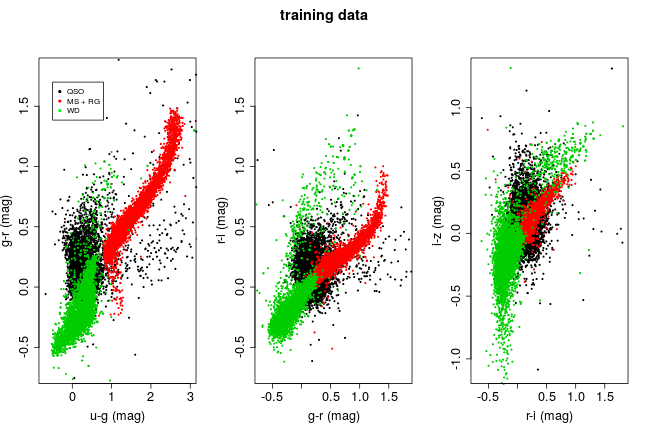
There are a few interesting features here. Firstly, there are hardly any white dwarfs identified. This could be because there aren’t very many in this data set, or the algorithm is failing to pick up on them. In the u-g/g-r plot on the left hand side their is also a clear vertical boundary on the red stellar classification. This lines up exactly with where the stars with lowest u-g line ratio lie in the training set, suggesting that our model isn’t able to classify stars beyind this range.
Given that we don’t know what is actually in the ‘test’ data set, it’s hard to draw any firm conclusions from it, but it does highlight some of the limitations of such learning algorithms, namely that they are very bad at predicting events beyond what they’ve been trained to; this is more generally known as ‘overfitting’, in relation to the training set.
All of the code used to produce this post is available here. Thanks for reading.
Subscribe via RSS